Equal Earth, from a world map to the mathematics

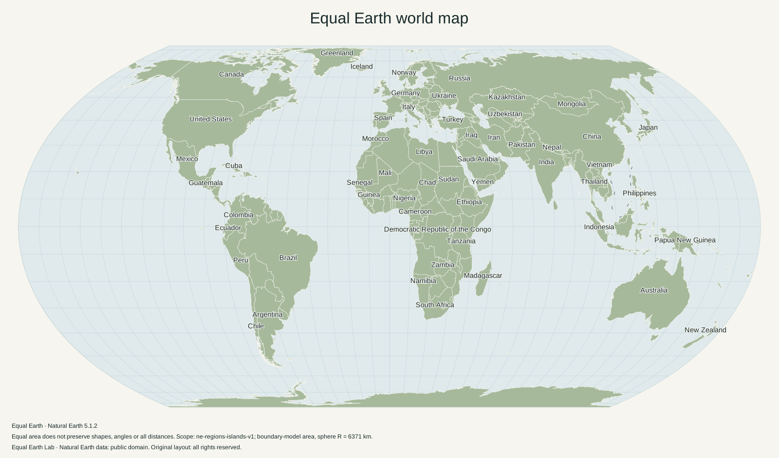
The claim behind the picture

Equal Earth is an equal-area projection of the world. Draw two regions with the same geographic area, apply its equations at the same scale, and the two filled regions have the same map area. They need not have the same shape, orientation, width or height. This is a much stronger statement than saying that the continents look approximately right.

The projection was designed by Bojan Šavrič, Tom Patterson and Bernhard Jenny. Their original paper was published online in 2018. Its appearance draws on Robinson, but it meets a different geometric requirement: Robinson is a compromise projection, while Equal Earth is mathematically area-preserving.

This article develops the spherical version used by the maps on this site. The proof and numerical examples below are worked explanations of the published equations. They are not a claim that the Earth is a perfect sphere, nor that every digital boundary is exact. Those are separate modelling questions, which become important when interpreting the displayed numbers.

Start with area on the sphere

Let λ be longitude measured east or west of the map’s central meridian. Let φ be latitude, and let R be the sphere’s radius. Angles in the equations are in radians. One degree is π / 180 radians; forgetting that conversion produces an entirely different map.

A tiny north–south step of dφ has length R dφ. A tiny east–west step of dλ at latitude φ has length R cos φ dλ. The cosine appears because a parallel of latitude is smaller than the equator. Multiplying the two perpendicular lengths gives the tiny patch’s spherical area:

Sphere area element = R² cos φ dλ dφ

This equation explains a familiar trap. A box covering ten degrees of longitude and ten degrees of latitude is not an equal-area box everywhere on Earth. Close to a pole, the longitude lines converge and the box becomes much narrower on the ground. Counting grid cells on a rectangular longitude–latitude image therefore does not directly measure geographic area.

An equal-area projection has to compensate for this changing ground width. Its job is not to make all longitude–latitude cells equally large. Its job is to make each cell’s map area proportional to its actual area on the sphere.

The forward equations

Equal Earth uses an auxiliary angle θ to make the equations manageable. First define M and θ, then a polynomial F and its derivative D:

M = √3 / 2
θ = arcsin(M sin φ)

F(θ) = A₁θ + A₂θ³ + A₃θ⁷ + A₄θ⁹
D(θ) = A₁ + 3A₂θ² + 7A₃θ⁶ + 9A₄θ⁸

A₁ =  1.340264
A₂ = −0.081106
A₃ =  0.000893
A₄ =  0.003796

The projected coordinates are:

x = R λ cos θ / [M D(θ)]
y = R F(θ)

These are the published coefficients and spherical equations, also visible in the PROJ implementation and D3’s Equal Earth source. The grouping with F and D is used here to expose the relationship between the vertical coordinate and the horizontal scale.

The y coordinate depends only on latitude. That is why every parallel is a horizontal line. At a fixed latitude, x is proportional to longitude, so meridians are evenly spaced along that parallel. The multiplier changes with latitude, causing the outer meridians to curve. The central meridian has λ = 0 and therefore x = 0 at every latitude.

The auxiliary angle also explains the finite poles. At geographic latitude 90°, θ is arcsin(√3 / 2), or 60°. The polynomial is evaluated at a finite argument; no logarithm or division by cos φ sends y to infinity. The north and south poles become finite line segments in the flat representation. Geographic longitude is undefined at the exact pole, so those segments should be understood as the projection’s limiting boundary, not as a physical length on Earth.

A direct proof that area is preserved

The local area multiplier of a coordinate transformation is its Jacobian determinant. For a map from longitude and latitude to x and y, the determinant is:

J = (∂x/∂λ)(∂y/∂φ) − (∂x/∂φ)(∂y/∂λ)

Because y depends only on φ, its longitude derivative is zero. The second term disappears. We only need the two derivatives in the first term.

Differentiate sin θ = M sin φ. The chain rule gives:

cos θ · dθ/dφ = M cos φ

dθ/dφ = M cos φ / cos θ

Since D is the derivative of F, differentiating the map’s y coordinate gives:

∂y/∂φ = R D(θ) M cos φ / cos θ

Longitude appears linearly in x, so:

∂x/∂λ = R cos θ / [M D(θ)]

Multiplying these expressions cancels D, M and cos θ:

J = R² cos φ

Map area element = |J| dλ dφ
                 = R² cos φ dλ dφ
                 = Sphere area element

That equality is the result we needed. For every regular interior point of the map, an infinitesimal spherical patch and its projected patch have the same area in the corresponding squared units. Applying one display scale multiplies every map area by the same constant, leaving all area ratios intact.

To move from a tiny patch to an entire country, integrate these area elements over the country’s region. Because the elements agree throughout the interior, their sums agree too. The map’s cut and its exact pole boundary require special handling in rendering, but they do not add a positive area of land. A correct renderer splits features at the cut and retains all their pieces.

Notice what the proof did not require. It did not require a particular country’s outline or a calibration against Africa and Greenland. The guarantee comes from the transformation itself. Any sufficiently well-defined region follows the same rule.

A worked rectangle example

For a longitude–latitude rectangle between longitudes λ₁ and λ₂ and latitudes φ₁ and φ₂, integration gives a convenient reference area:

Area = R² (λ₂ − λ₁) (sin φ₂ − sin φ₁)

Suppose the rectangle spans 10° of longitude and runs from 0° to 10° north. On a sphere of radius 6,371 km, this formula gives about 1.23 million km². Move a rectangle with the same angular width and height to 60°–70° north and its area falls to about 522,000 km². The second rectangle is geographically smaller because its east–west sides lie on shorter parallels.

Equal Earth must show that smaller area. A pair of rectangles that occupy identical numbers of degrees are not a valid visual test for equal-area behaviour. The test must use regions whose spherical areas are equal, such as circles with the same angular radius, or an identical polygon moved by a rigid rotation on the sphere.

This distinction is also important in software. Replacing a country’s latitude with latitude plus ten degrees for every vertex does not rigidly move the country. It changes the distances between vertices because longitude degrees have different lengths at the new latitude. The area may change before the projection even begins.

The movable country outlines on the world map use a spherical rotation instead. The same region is reoriented on the globe and then projected again. That preserves the source region’s spherical area while allowing its flat appearance to change.

Why shapes can still be wrong

Preserving area constrains a product, not each separate length. A local transformation can stretch a small patch by a factor of two in one principal direction and compress it by one half in the perpendicular principal direction. The product remains one, although a circle becomes an ellipse.

For a more precise description, express the local transformation in orthonormal east and north directions on the sphere. Its two principal scale factors, often called the singular values of that local matrix, describe maximum and minimum stretching. For an equal-area projection, their product is one. Neither factor has to equal one individually.

Away from the central meridian, the directions of greatest stretching need not align with east and north. Looking only at the spacing of latitude lines therefore misses part of the distortion. The term ∂x/∂φ, which vanished from the area determinant because ∂y/∂λ is zero, still matters to shape and angle distortion.

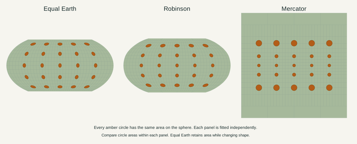
Every amber patch in this figure began as a circle of angular radius 5° on the sphere. They are finite circles rather than infinitesimal mathematical indicators, so the figure is a visual illustration of local distortion. Within Equal Earth’s panel, the projected patches retain equal areas even where their shapes become slanted or flattened. The three panels use independently fitted display scales; the useful comparison is the pattern within each map.

A practical consequence follows. An Equal Earth outline may look wider at one longitude than at another without gaining area. The compensating change may be in height, tilt or the shape of different parts of the outline. A bounding box is not a measurement of the country’s filled area.

Equal Earth versus Mercator in one equation

For spherical Mercator, local linear scale relative to the equator is 1 / cos φ in every direction. The area factor is the square of that scale:

Mercator local area factor = 1 / cos² φ
Equal Earth local area factor = 1

Latitude	Equal Earth area factor	Mercator area factor
0°	1.00	1.00
30°	1.00	1.33
45°	1.00	2.00
60°	1.00	4.00
80°	1.00	33.16

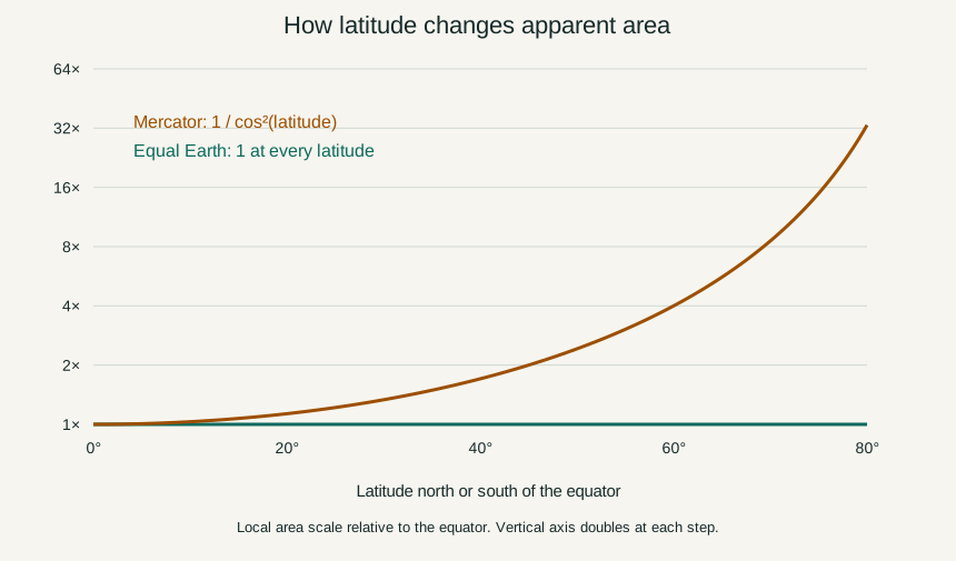
These figures describe very small patches at the stated latitude. They do not mean that every country touching 60° is four times too large in Mercator. A whole-country factor would require integrating Mercator’s changing area multiplier across the country’s complete geography, including any separated islands.

Mercator’s matching scale in every local direction is what preserves local angles. Equal Earth’s balanced stretching and compression preserve area instead. Neither statement means that a ruler measures all globe distances correctly on the resulting world map.

Finding latitude and longitude from a map point

Interactive maps need the inverse transformation too. A pointer supplies screen coordinates; selecting a destination requires geographic coordinates. Equal Earth’s forward y equation is a ninth-degree polynomial in θ, and a practical inverse solves it numerically.

Remove any screen translation and uniform display scale first. Divide the map coordinates by R, giving normalized X and Y. Start with a reasonable θ estimate and apply Newton’s method:

θ(next) = θ − [F(θ) − Y] / D(θ)

Each step subtracts the vertical error divided by the current slope. Once the change is sufficiently small, recover latitude and longitude:

φ = arcsin(sin θ / M)
λ = X M D(θ) / cos θ

The implementation must still reject points outside the projection’s curved outline. A numerical inverse returning finite numbers does not by itself prove that a screen point belongs to the valid map. Forward-projecting the recovered position and checking that it returns to the original point is one useful validation.

Longitude then needs to be interpreted relative to the selected central meridian. The same geographic location can appear close to one map edge or near the centre after recentering. A screen coordinate is therefore meaningful only together with the projection, centre, orientation, scale and translation that produced it.

The sphere, the ellipsoid and the pixels

The proof above is exact for its stated sphere. A reference ellipsoid has a different area element. The authors describe using an authalic latitude transformation for the ellipsoidal version, and PROJ supports spherical and ellipsoidal Equal Earth. Authalic conversion transfers the ellipsoid to an equal-area sphere before the spherical projection is applied.

Equal Earth Lab uses one explicit spherical model for comparisons. That keeps country geometry, area calculations and spherical relocation consistent. The resulting figures can differ from official statistics that use a different Earth model, inland-water definition, coastline resolution or territorial scope. Printing more decimal places would not remove those differences.

A browser also does not draw a continuous mathematical surface. It draws line segments and pixels. Coastlines may be simplified for speed; curves are subdivided; antialiasing gives edge pixels partial colour. Counting coloured screen pixels can therefore produce a small numerical discrepancy even when the projection equations are correct.

The right validation separates these layers. Check the analytic area property; compare projected polygon area with spherical polygon area using adequate precision; inspect cut-line and polar cases; and verify that the display has not independently resized each compared object. Two equal-area silhouettes fitted separately into equal boxes lose their useful common area scale.

What to do with this knowledge

Choose Equal Earth when relative geographic area is part of your message. Use the country comparisons to see the consequence on complete outlines, and move a comparison copy on the world map to examine spherical relocation. A global area comparison is strongest when the boundary scopes and the numerical model are stated alongside the map.

Choose a different representation when another property takes priority. The Mercator reference explains local angles and constant-bearing lines. The Robinson reference explains a compromise designed around the appearance of the whole world. Their strengths are clearer when the property being preserved is named explicitly.

Equal Earth’s main achievement is not the elimination of every map distortion. Its equations make a specific promise about area, and the Jacobian calculation shows exactly why that promise holds. Knowing both the promise and its limits makes the resulting world map much easier to read honestly.